This is the fourth post in my series on some simple kanban board statistics. We have been talking about:
And this time it’s time to see if we can visualize a bit where time is spent. For this first post, we will make some basic classifications of active and not active or not “on the board” and “on the board”.
In the coming posts I want to expand on this and see if we can make a distinction between other states on the board as well, but for that, we need to expand the data in “Raw data”, because that data only contains completed items right now.
Ok - let’s get going. As for all these post I am in this Google Sheet - make a copy if you want to play along
The dates
There are three dates that are important for these calculations:
- Created Date - the date when the ticket was created.
- Activated Date - the date when work was started on the ticket.
- Closed Date - the date the ticket (first) was closed.
Closed Date - Start Date = lead time as we said before.
But we never used the Activation date. And with that we can get two more data points:
Activation date - Start date = time in backlog. This is the time from when the ticket was created and until we started to work on it. Typically tickets spend a lot of time waiting in the backlog before we start to work on them. I’ve written several times, about the bad things a long backlog brings that it brings with it, but here’s a way to show this in numbersClosed date - Activation Date = time on board. This gives us the time when the ticket has been on the board. That doesn’t necessarily mean that we worked with it (it can have been blocked or down prioritized etc.), but at least it’s in been under our attention.- Also, we can get a chance to see how big part of the lead time that is made up of waiting respectively working.
In later posts, we can count stuff that is still in the backlog, but we can do that now since that data is not included yet.
I was lucky, in one regard, since the electronic system I used (Team Foundation Service), at my current client, have an “Activation date” ready. In JIRA this date might be trickier to get hold of, but there is a “Date started” field that can prove useful.
The data
As before, I’m going to make a new tab “Time spent distributions” and do all my calculations there.
We need to calculate the date and differences per item so let’s bring up our old friend the QUERY-function and write the following:
=QUERY('Raw data'!A2:I, "SELECT A,G,H,I WHERE G<>I AND I IS NOT NULL ORDER BY I")
This will select all the items that:
-
has different dates for Created and Closed date - meaning not the ones we closed on the same day we created them. Or in other words; has a lead time above 0 days.
-
and has a closed date (which are all rows now, but just you wait…)
I selected the ID, Created, Activation and Closed dates as we will need them.
I put this formula in A2 as I wanted a header row over the data.
It’s now pretty easy to calculate the time spent in each stage:
- In column E: Lead time =
Closed date - Created date - In column F: In backlog =
Activated date - Created date - In column G: On board =
Closed date - Activated date
For future use, I’ve also added the month and week when the item was closed.
Squinting chart
Let me show one chart that could be useful; I call it the squinting chart.
- Select columns ID, “In backlog” and “On board”
- Create a 100% stacked bar chart
- Set a proper Chart title and put the legend on the bottom
You will get something that looks like this:
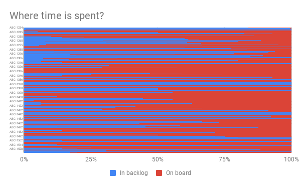
Yes, that is messy, but if you squint your eyes… is it more red or blue? More red, right? Meaning that most of our time is spent on the board, not in the backlog, as I thought. Interesting, but a bit messy maybe.
Let’s see how much and how that trend is moving
How about the trend then?
I now did a similar thing as we did for the throughput in the last post: let’s aggregate the averages per month and week and see if that gives us anything interesting.
I will show you what I did for weeks, but it’s quite similar for months.
- Create a list of UNIQUE-formula for weeks
=UNIQUE(I2:I). I put mine inO2 - Calculate the average number of days “In backlog”, in Column P, for that month, using this formula
=AverageIf(I2:I, O2, F2:F). Here’s a breakdown of the arguments to the formula- Find the rows in
I2:I(Closed date) that - matches the value in
O2 - And make an average of the
F2:Fvalues
- Find the rows in
- I then repeated for a “Average On Board”-column:
=AverageIf($I$2:I, O2, $G$2:G)- The
$will lock that reference when you fill the rows for all the unique weeks.
- The
- Finally, I added a total time, or “Average lead time” by just adding “In backlog” and “On board”
- And filled the formulas for all the rows.
- Pro tip for fast filling:
- Select the formulas you want to fill
P2:R2in our case - Double click the little handle in the bottom corner
- Google sheets will auto-fill the formulas for all the rows of unique weeks
- This is when the
$for locking certain references comes handy as Google sheets otherwise will increment row references…
- Select the formulas you want to fill
- Pro tip for fast filling:
Ok - that data looks fine! But let’s show it as well.
For the months I created a simpler chart; a stacked column chart for K1:M7 (columns Unique month, Average In Backlog and Average On Board). A nifty little setting was where you can set a label, per column, for the total. The result looks like this:
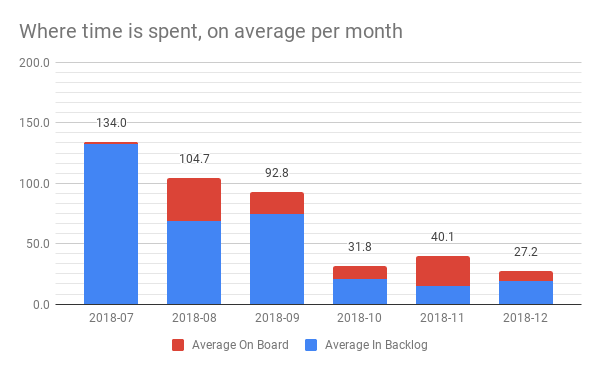
Ok - that was pretty and shows that the total lead time goes down. And time on board goes up, percentage-wise. Nice. That’s good, but let’s become more granular.
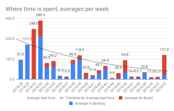
For the weeks I made a Combo chart (whatever that means) out of the O:R columns, with unique weeks, average in backlog on board and the lead time. Here’s how it will look when we are done:
- Edit the chart and select Stacking = Standard as we want the columns to be stacked on top of each other
- Now open the Customize tab
- Go to the series setting and select the Average in Backlog series.
- Make sure it’s set on Columns
- Repeat for the Average On board
- Now select the Lead time series and make it a line. (AH! This is what a combo chart is). That will be the top of each column (as lead time is the sum of In backlog and On board), so this line is not particularly interesting
- However, the trend of the average lead time is pretty interesting.
- Check the box for trend line (i used a moving average to smooth the trend line out a bit) and format it in some nice way
- Now, let’s remove the actual line by selecting Color = None
- Done - admire your work
Ha! Pretty useful chart actually. We see both the total lead time and its trend (falling steadily for this team) as well as where the time is spent.
Summary
In this post we charted out where the time for this data was spent; in the backlog or on the board. We used a few different chart types to do this and still didn’t touch the raw data.
In the next post, I will try to make a few static numbers that people often ask about and that we, relatively easily can pull from the data.
Here’s a final link to the Google Sheet I’m working in. Feel free to copy it if you find this useful.
The links
My sheet is open for anyone to read and, if you want to, make a copy of. If you use it and find it useful - please throw me an attribution or a nice thought. If you make something awesome out of it - please let me know so that I can learn more about this.
All the posts in the series are found through these links: